What is an IP address?
Computers communicate over the Internet using the
IP protocol (
Internet Protocol), which uses numerical addresses, called
IP addresses, made up of four whole numbers (4
bytes) between 0 and 255 and written in the format xxx.xxx.xxx.xxx. For example,
194.153.205.26 is an IP address given in technical format.
These addresses are used by networked computers to communicate, so each computer on a network has a unique IP address on that network.
It is ICANN (
Internet Corporation for Assigned Names and Numbers, replaced since 1998 by IANA,
Internet Assigned Numbers Agency) which is responsible for allocating public IP addresses, i.e. IP addresses for computers directly connected to the public internet network.
Decrypting an IP address
An
IP address is a
32 bit address, generally written in the format of 4 whole numbers separated by dots. There are two distinct parts to an IP address:
- the numbers to the left indicate the network and are called the netID,
- the numbers to the right indicate the computers on this network and are called the host-ID.
Shown in the example below:
Note the network to the left 194.28.12.0. It contains the following computers:
- 194.28.12.1 to 194.28.12.4
Note that of the right 178.12.0.0. It includes the following computers:
- 178.12.77.1 to 178.12.77.6
In the case above, the networks are written 194.28.12 and 178.12.77, then each computer making up the network is numbered incrementally.
Take a network written 58.0.0.0. The computers on this network could have IP addresses going from 58.0.0.1 to 58.255.255.254. So, it is a case of allocating the numbers in such a way that there is a structure in the hierarchy of the computers and servers.
So, the smaller the number of bits reserved on the network, the more computers it can contain.
In fact, a network written
102.0.0.0 can contain computers whose IP address can vary between 102.0.0.1 and 102.255.255.254 (256*256*256-2=16,777,214 possibilities), while a network written
194.24 can only contain computers where the IP address is between 194.26.0.1 and 194.26.255.254 (256*256-2=65,534 possibilities), this is the notion of
IP address classes.
Special addresses.
When the host-id is cancelled, i.e. when the bits reserved for the machines on the network are replaced by zeros (for example 194.28.12.0), something called a network address is obtained. This address cannot be allocated to any of the computers on the network.
When the netid is cancelled, i.e. when the bits reserved for the network are replaced by zeros, a machine address is obtained. This address represents the machine specified by the host-ID which is found on the current network.
When all the bits of the host-id are at 1, the address obtained is called the broadcast address. This a specific address, enabling a message to be sent to all the machines on the network specified by the netID.
Conversely, when all the bits of the netid are at 1, the address obtained is called the multicast address.
Finally the address
127.0.0.1 is called the
loopback address because it indicates the
localhost.
Network classes
IP addresses are divided into classes, according to the number of bytes which represent the network.
Class A
In a class A IP address, the first byte represents the network.
The most significant bit (the first bit, that to the left) is at zero which means that there are 27 (00000000 to 01111111) network possibilities, which is 128 possibilities However, the 0 network (bits valuing 00000000) does not exist and number 127 is reserved to indicate your machine.
The networks available in class A are therefore networks going from 1.0.0.0 to 126.0.0.0 (the last bytes are zeros which indicate that this is indeed a network and not computers!)
The three bytes to the left represent the computers on the network, the network can therefore contain a number of computers equal to:
224-2 = 16,777,214 computers.
A class A IP address, in binary looks like:
Class B
In a class B IP address, the first two bytes represent the network.
The first two bits are 1 and 0, which means that there are 214 (10 000000 00000000 to 10 111111 11111111) network possibilities, which is 16,384 possible networks. The networks available in class B are therefore networks going from 128.0.0.0 to 191.255.0.0.
The two bytes to the left represent the computers on the network. The network can therefore contain a number of computers equal to:
216-21 = 65,534 computers.
A class B IP address, in binary looks like:
Class C
In a class C IP address, the first three bytes represent the network. The first three bits are 1,1 and 0 which means that there are 221 network possibilities, i.e. 2,097,152. The networks available in class C are therefore networks going from 192.0.0.0 to 223.255.255.0.
The byte to the left represents the computers on the network, the network can therefore contain:
28-21 = 254 computers.
In binary, a class C IP address looks like:
Allocation of IP addresses
The aim of dividing IP addresses into three classes A, B and C is to make the search for a computer on the network easier. In fact, with this notation it is possible to firstly search for the network that you want to reach, then search for a computer on this network. So, allocation of IP address is done according to the size of the network.
Class A addresses are used for very large networks, while class C addresses are for example allocated to small company networks.
Reserved IP addresses
It frequently happens that in a company or organisation only one computer is linked to the Internet and it is through this that other computers on the network access the Internet (generally we talk of a
proxy or gateway).
In such a case, only the computer linked to the network needs to reserve an IP address with ICANN. However, the other computers still need an IP address to be able to communicate with each other internally.
So, ICANN has reserved a handful of addresses in each class to enable an IP address to be allocated to computers on a local network linked to the Internet without the risk of creating IP address conflicts on the network of networks. These are the following addresses:
- Private class A IP addresses: 10.0.0.1 to 10.255.255.254, enabling the creation of large private networks comprising of thousands of computers.
- Private class B IP addresses: 172.16.0.1 to 172.31.255.254, making it possible to create medium sized private networks.
- Private class C IP addresses: 192.168.0.1 to 192.168.0.254, for putting in place small private networks.
Subnet masks
Subnet masks
In short, a mask is produced containing 1s with the location of bits that you want to keep and 0s for those you want to cancel. Once this mask is created, you simply put a logical AND between the value you want to mask and the mask in order to keep the part you wish to cancel separate from the rest.
So a
netmask is presented in the form of 4 bytes separated by dots (like an IP address), it comprises (in its binary notation) zeros at the level of the bits from the IP address that you wish to cancel (and ones at the level of those you want to keep).
Importance of subnet masks
The primary importance of a subnet mask is to enable the simple identification of the network associated to an IP address.
Indeed, the network is determined by a certain number of bytes in the IP address (1 byte for class A addresses, 2 for class B and 3 bytes for class C). However, a network is written by taking the number of bytes which characterise it, then completing it with zeros. For example, the network linked to the address 34.56.123.12 is 34.0.0.0, because it is a class A type IP address.
To find out the network address linked to the IP address 34.56.123.12, you simply need to apply a mask where the first byte is only made up of 1s (which is 255 in decimal), then 0s in the following bytes.
The mask is: 11111111.00000000.00000000.00000000
The mask associated with the IP address 34.208.123.12 is therefore 255.0.0.0.
The binary value of 34.208.123.12 is: 00100010.11010000.01111011.00001100
So an AND logic between the IP address and the mask gives the following result:
00100010.11010000.01111011.00001100
  AND
11111111.00000000.00000000.00000000
  =
00100010.00000000.00000000.00000000
Which is
34.0.0.0. It is the network linked to the address
34.208.123.12
By generalising, it is possible to obtain masks relating to each class of address:
- For a Class A address, only the first byte must be retained. The mask has the following format 11111111.00000000.00000000.00000000, i.e. 255.0.0.0 in decimal;
- For a Class B address, the first two bytes must be retained, which gives the following mask 11111111.11111111.00000000.00000000, relating to 255.255.0.0 in decimal;
- For a Class C address, by the same reasoning, the mask will have the following format 11111111.11111111.11111111.00000000, i.e. 255.255.255.0 in decimal;
Creation of subnets
Let us re-examine the example of the network 34.0.0.0, and assume that we want the first two bits of the second byte to make it possible to indicate the network.
The mask to be applied will then be:
11111111.11000000.00000000.00000000
That is 255.192.0.0
If we apply this mask to the address 34.208.123.12 we get:
34.192.0.0
In reality there are 4 possible scenarios for the result of the masking of an IP address of a computer on the network 34.0.0.0
- When the first two bits of the second byte are 00, in which case the result of the masking is 34.0.0.0
- When the first two bits of the second byte are 01, in which case the result of the masking is 34.64.0.0
- When the first two bits of the second byte are 10, in which case the result of the masking is 34.128.0.0
- When the first two bits of the second byte are 11, in which case the result of the masking is 34.192.0.0
Therefore, this masking divides a class A network (able to allow 16,777,214 computers) into 4 subnets - from where the name of subnet mask - can allow 222 computers or 4,194,304 computers.
It may be interesting to note that in these two cases, the total number of computers is the same, which is 16,777,214 computers (4 x 4,194,304 - 2 = 16,777,214).
The number of subnets depends on the number of additional bits allocated to the network (here 2). The number of subnets is therefore:

Concept of IPV4 By Russ White.
IP addresses, both IPv4 and IPv6, appear to be complicated when you first encounter them, but in reality they are simple constructions, and a using a few basic rules will allow you to find the important information for any situation very quickly—and with minimal math. In this article, we review some of the basics of IPv4 address layout, and then consider a technique to make working with IPv4 addresses easier. Although this is not the “conventional” method you might have been taught to work with in IP address space, you will find it is very easy and fast. We conclude with a discussion of applying those techniques to the IPv6 address space.
Basic Addressing
IPv4 addresses are essentially 32-bit binary numbers; computer systems and routers do not see any sorts of divisions within the IPv4 address space. To make IPv4 addresses more human-readable, however, we break them up into four sections divided by dots, or periods, commonly called “octets.” An octet is a set of eight binary digits, sometimes also called a “byte.” We do not use byte here, because the real definition of a byte can vary from computer to computer, whereas an octet remains the same length in all situations. Figure 1 illustrates the IPv4 address structure.

Figure 1: IPv4 Address Structure
Because each octet represents a binary (base 2) number between 0 and 2
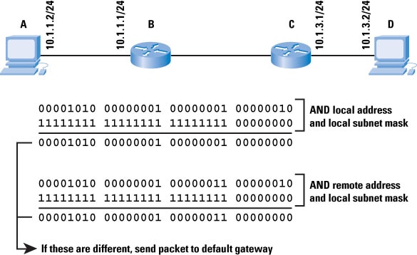
8, each octet will be between 0 and 255. This part of IPv4 addresses is simple—but what about subnet masks? To understand a subnet mask, we need to understand how a device actually uses subnet masks to determine where to send a specific packet, as Figure 2 illustrates.
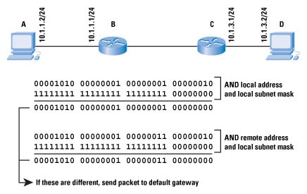
Figure 2: Subnet Masks
If host A, which has the local IP address
10.1.1.2 with a subnet mask of
255.255.255.0, wants to send a packet to
10.1.3.2, how does it know whether D is connected to the same network (broadcast domain) or not? If D is connected to the same network, then A should look for D’s local Layer 2 address to transmit the packet to. If D is not connected to the same network, then A needs to send any packets destined to D to A’s local default gateway.
To discover whether D is connected or not, A takes its local address and performs a logical AND between this and the subnet mask. A then takes the destination (remote) address and performs the same logical AND (using its local subnet mask). If the two resulting numbers, called the
network address or
prefix, match, then the destination must be on the local segment, and A can simply look up the destination in the
Address Resolution Protocol (ARP) cache, and send the packet locally. If the two numbers do not match, then A needs to send the packet to its default gateway.
Note: ARP is a protocol used to discover the mappings between the IP addresses of devices attached to the same network as the local device and the Layer 2 address of devices attached to the same network as the local device. Essentially, a device sends an ARP broadcast containing the IP address of some other device it believes to be connected, and the device with the specified IP address replies with its Layer 2 address, providing a mapping between these two addresses.
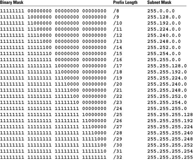
If a subnet mask is a “dotted decimal” version of the binary subnet mask, then what is the prefix length? The prefix length is just a shorthand way of expressing the subnet mask. The prefix length is the number of bits set in the subnet mask; for instance, if the subnet mask is
255.255.255.0, there are 24 1’s in the binary version of the subnet mask, so the prefix length is 24 bits. Figure 3 illustrates network masks and prefix lengths.

Figure 3: Prefix Lengths
Working with IPv4 Addresses
Now that we understand how an IPv4 address is formed and what the subnet length and prefix length are, how do we work with them? The most basic questions we face when working with an IP address follow:
- What is the network address of the prefix?
- What is the host address?
There are two ways to find the answers to these questions: the hard way and the easy way. We cover the hard way first, and then show you the easy way.
The Hard Way
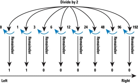
The hard way to determine the prefix and host addresses is to convert the address into binary, perform logical AND and NOR operations on the address and the subnet mask, and then convert the resulting numbers back to decimal. Figure 4 illustrates the process of converting a single octet of the IPv4 address into binary; the number converted in this case is 192.
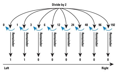
Figure 4: Binary Conversion
The process is simple, but tedious; divide the octet value by 2, take the remainder off, and then divide by 2 again, until you reach 0. The remainders, reversed in direction, are the binary numbers representing the value of the octet. Performing this process for all four octets, we have the binary IP address, and can use logical AND and NOR operations to find the prefix (network address) and the host address, as Figure 5 shows for the address
192.168.100.80/26.
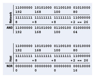
Figure 5: Address Calculation
The Easy Way
All this conversion from binary to decimal and from decimal to binary is tedious— is there an easier way? Yes. First, we start with the observation that we work only with the numbers within one octet at a time, no matter what the prefix length is. We can assume all the octets before this
working octet are part of the network address, and octets after this
working octet are part of the host address.
The first thing we need to do, then, is to find out which octet is our
working octet. This task is actually quite simple: just divide the prefix length by 8, discard the remainder, and add 1. The following table provides some examples.
Note: Another way to look at this task is that you will ignore the octets indicated by the division. For instance, for 192.168.100.80/26, the result of dividing 26 by 8 is 3, so you will ignore the first three octets of the IP address, and work only with the fourth octet. This process has the same result.
When we know the working octet, what do we do with it? Well, we could simply use the procedure outlined, convert the single octet to binary, perform AND and NOR operations on it with the right bits from the subnet mask, and then put it all back together to find the network and host addresses—but there is an easier way to find the network and host parts of the working octet. Start by doing the same math, only this time we want to work with the remainder rather than the result.
192.168.100.80/26
26 ÷ 8 = 3 with a remainder of 2
Take the remainder, and use the following table to find the corresponding
jump within the octet; this number is the distance, in decimal form, between the network addresses within the octet.
In this chart, the first column represents the prefix length
within this octet, the second column represents the prefix value when this bit is set to 1, the number of hosts in the subnet for this prefix length, and the
jump between network addresses with the specified prefix length.
The number 2 corresponds to 64, so the jump is 64—there is a network at 0, 64, 128, 192, and 224 in this octet. Now all we need to do is figure out which one of those networks this address is in. This task is fairly simple: just take the largest network number that fits into the number in the working octet. In this case, the largest number that fits into 80 is 64, so our network address is
192.168.100.64/26.
Now, what about the host address? That is easy when we have the network address—just subtract the network address from the IP address, and you have the host address within the network: 80 – 64 = 16. This process takes a little practice, but it is not hard when you become accustomed to the steps.
In the second and third examples, you see that the working octet is actually the third, rather than the fourth, octet. To find the host address in these examples, you simply find the host address in the third octet, and then “tack on” the fourth octet as part of the host address as well, because part of the third octet—and all of the fourth octet—are actually part of the host address.
Summarization and Subnets
Subnets and supernets are probably the hardest part of IP addressing for most people to understand and handle quickly, but they are both based on a very simple concept—
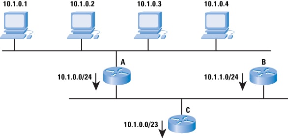
aggregation. Figure 6 shows how aggregation works.
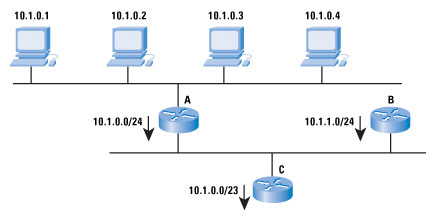
Figure 6: Address Aggregation
The figure shows four hosts with the addresses
10.1.0.1, 10.1.0.2, 10.1.0.3, and
10.1.0.4. Router A advertises
10.1.1.0/24, meaning: “Any host within the address range
10.1.0.0 through
10.1.0.255 is reachable through me.” Note that not all the hosts within this range exist, and that is okay—if a host within that range of addresses is reachable, it is reachable through Router A. In IP, the address that A is advertising is called a
network address, and you can conveniently think of it as an address for the wire the hosts and router are attached to, rather than a specific device.
For many people, the confusing part comes next. Router B is also advertising
10.1.1.0/24, which is another network address. Router C can combine—or aggregate—these two advertisements into a single advertisement. Although we have just removed the correspondence between the wire and the network address, we have not changed the fundamental meaning of the advertisement itself. In other words, Router C is saying: “Any host within the range of addresses from
10.1.0.0 through
10.1.1.255 is reachable through me.” There is no wire with this address space, but devices beyond Router C do not know this, so it does not matter.
To better handle aggregated address space, we define two new terms,
subnets and
supernets. A subnet is a network that is contained entirely within another network; a supernet is a network that entirely contains another network. For instance,
10.1.0.0/24 and
10.1.1.0/24 are both subnets of
10.1.0.0/23, whereas
10.1.0.0/23 is a supernet of
10.1.0.0/24 and
10.1.1.0/24.
Now we consider a binary representation of these three addresses, and try to make more sense out of the concept of aggregation from an addressing perspective; Figure 7 illustrates.
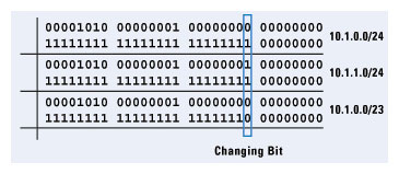
Figure 7: Aggregation Details
By looking at the binary form of
10.1.0.0/24 and
10.1.1.0/24, we can see that only the 24th bit in the network address changes. If we change the prefix length to 23, we have effectively “masked out” this single bit, making the
10.1.0.0/23 address cover the same address range as the
10.1.0.0/24 and
10.1.1.0/24 addresses combined.
The Hardest Subnetting Problem
The hardest subnetting problem most people face is that of trying to decide what the smallest subnet is that will provide a given number of hosts on a specific segment, and yet not waste any address space. The way this sort of problem is normally phrased is something like the following:
You have 5 subnets with the following numbers of hosts on them: 58, 14, 29, 49, and 3, and you are given the address space 10.1.1.0/24. Determine how you could divide the address space given into subnets so these hosts fit into it.
This appears to be a very difficult problem to solve, but the chart we used previously to find the jump within a single octet actually makes this task quite easy. First, we run through the steps, and then we solve the example problem to see how it actually works.
- Order the networks from the largest to the smallest.
- Find the smallest number in the chart that fits the number of the largest number of hosts + 2 (you cannot, except on point-to-point links, use the address with all 0’s or all 1’s in the host address; for point-to-point links, you can use a /31, which has no broadcast addresses).
- Continue through each space needed until you either run out of space or you finish.
This process seems pretty simple, but does it work? Let’s try it with our example.
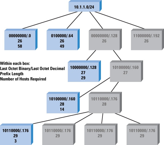
- Reorder the numbers 58, 14, 29, 49, 3 to 58, 49, 29, 14, 3.
- Start with 58.
- The smallest number larger than (58 + 2) is 64, and 64 is 2 bits.
- There are 24 bits of prefix length in the address space given; add 2 for 26.
- The first network is 10.1.1.0/26.
- The next network is 10.1.1.0 + 64, so we start the next “round” at 10.1.1.64.
- The next block is 49 hosts.
- The smallest number larger than (49 + 2) is 64, and 64 is 2 bits.
- There are 24 bits of prefix length in the address space given; add 2 for 26.
- We start this block at 10.1.1.64, so the network is 10.1.1.64/26.
- The next network is 10.1.1.64 + 64, so we start the next “round” at 10.1.1.128.
- The next block is 29 hosts.
- The smallest number larger than (29 + 2) is 32, and 32 is 3 bits.
- There are 24 bits of prefix length in the address space given; add 3 for 27.
- We start this block at 10.1.1.128, so the network is 10.1.1.128/27.
- The next network is 10.1.1.128 + 32, so we start the next “round” at 10.1.1.160.
- The next block is 14 hosts.
- The smallest number larger than (14 + 2) is 16, and 16 is 4 bits (actually equal, but it still works).
- There are 24 bits of prefix length in the address space given; add 14 for 28.
- We start this block at 10.1.1.160, so the network is 10.1.1.160/28.
- The next network is 10.1.1.160 + 16, so we start the next “round” at 10.1.1.176.
- The last block is 3 hosts.
- The smallest number larger than (3 + 2) is 8, and 8 is 5 bits.
- There are 24 bits of prefix length in the address space given; add 5 for 29.
- We start this block at 10.1.1.176, so the network is 10.1.1.176/29.
- This is the last block of hosts, so we are finished.
It is a simple matter of iterating from the largest to the smallest block, and using the simple chart we used before to determine how large of a
jump we need to cover the host addresses we need to fit onto the subnet. Figure 8 illustrates the resulting hierarchy of subnets.
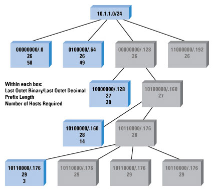
Figure 8: Subnet Chart
In this illustration:
- The first line in each box contains the final octet of the network address in binary and decimal forms.
- The second line in each box contains the prefix length.
- The third line indicates the number of hosts the original problem required on that subnet.
- Gray boxes indicate blocks of address space that are unused at that level.
Working with IPv6 Addresses
IPv6 addresses appear to be much more difficult to work with—but they really are not. Although they are larger, they are still made up of the same fundamental components, and hosts and routers still use the addresses the same way. All we really need to do is realize that each pair of hexadecimal numbers in the IPv6 address is actually an octet of binary address space. The chart, the mechanisms used to find the network and host addresses, and the concepts of super and subnets remain the same.
For example, suppose we have the IPv6 address
2002:FF10:9876: DD0A:9090:4896:AC56:0E01/63 and we want to know what the network number is (host numbers are less useful in IPv6 networks, because they are often the MAC address of the system itself).
- 63 ÷ 8 = 7, remainder 7.
- The working octet is the 8th, which is 0A.
- Remainder 7 on the chart says the jump is 2, so the networks are 00, 02, 04, 06, 08, 0A, 0C, and 0E.
- The network is 2002:FF10:9876:DD0A::/63.
The numbers are longer, but the principle is the same, as long as you remember that every
pair of digits in the IPv6 address is a single octet.